The 4 steps of a statistical analysis
Phase 1: ideal world (blinded to the data)
- Formulate the hypothesis/hypotheses to be tested.
- Define the population of interest for each hypothesis.
- Identify the variables/mecanisms that are related to each hypothesis:
- outcome(s), e.g. blood pressure after 1 week.
- exposure(s): e.g. therapy A vs B.
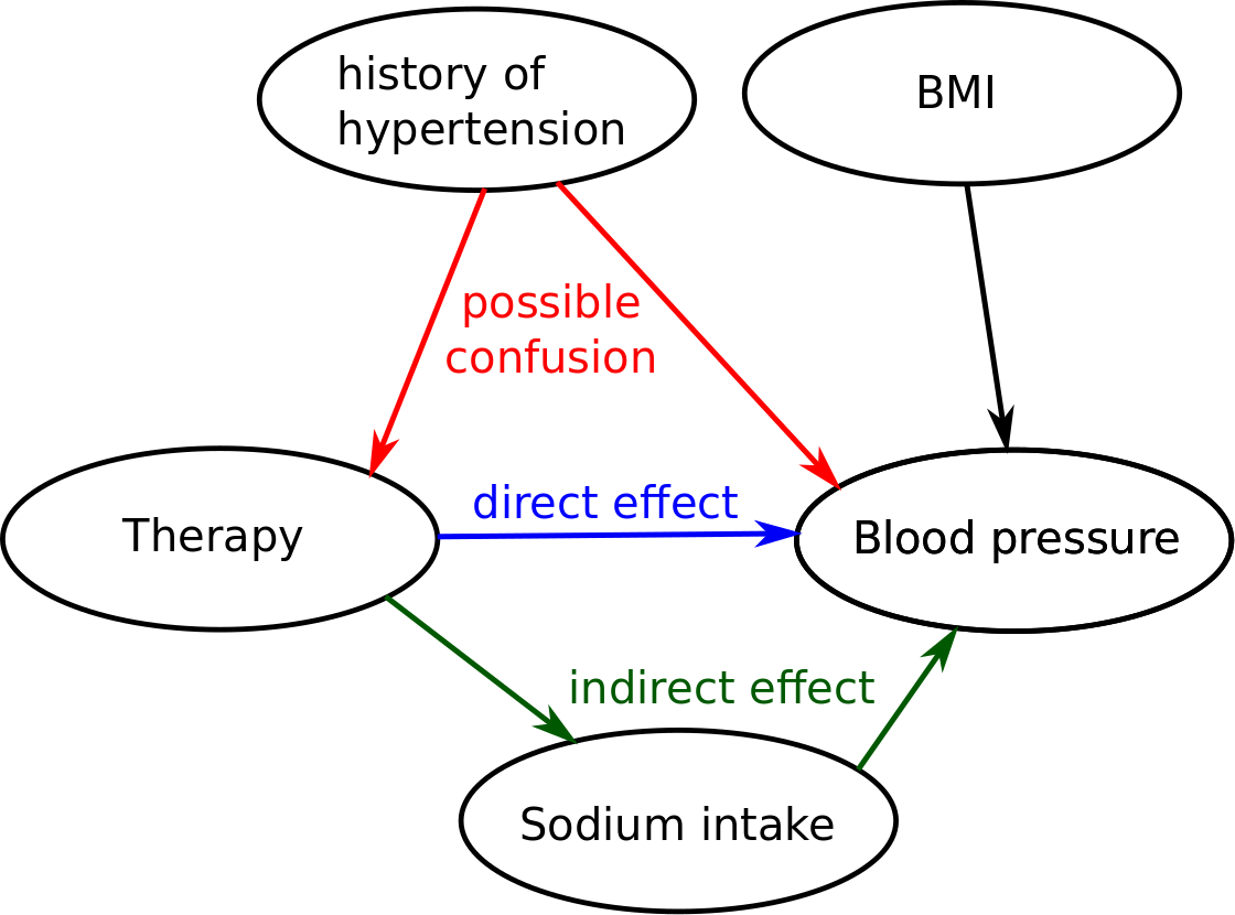
- confounder(s), e.g. history of hypertension, those patients are more likely to get therapy A.
- risk factor(s), e.g. BMI, therapy allocation is independent of BMI.
- mediators(s): sodium intake, therapy impacts both hypertension and sodium intake (sodium intake impacts hypertension).
-
Draw the causal graph
- What are the consequence of the design on the causal graph:
e.g. randomisation of the treatment allocation would remove the link between Therapy and history of hypertension.
e.g. a observational study could lead to have more confounders (doctor preferences could be related to Therapy and BMI).
e.g. a longitudinal study would induce a correlation between the mesurements of a blood pressure for a given individual. - The statistical model (or test) you will choose should reflect:
- the type of the outcome, e.g. binary -> logistic regression
- the design of your data, e.g. repetead measurements -> mixed model
- the causal graph: e.g. adjust for the possible confounders.
Phase 2: data management
- Work on the subset of data that is relevant for your analysis.
e.g. in some studies, people have collected more than 200 variables but in your study only 10 of them are relevant. Working on a smaller dataset ease the data checking. - Identify the individuals that will be kept for the study and create one dataset that will be used during the analysis. Drawing an inclusion and exlcusion is usually very usefull to understand and communicate how the individuals where selected.
- Check the data that have been collected, column by column.
Is there extreme/abnormal values? e.g. negative times, three levels for gender: “Male”, “male”, “Female”.
Does the univariate distributions match what you have expected? e.g. all patients have a blood pressure >130 mmHg - Name your variable in english. Never use special characters.
- Use explicit values and names for your variables.
e.g. gender = 0,1 is not good. It should be either Male = TRUE, FALSE or Gender = “Male”, “Female”. - Check that your data has been anonymized. You should however always keep an identification variable (e.g. Id = “Patient_1” to Id = “Patient_52”)
Phase 3: back to reality
Considering the data that you have collected:
- Does your dataset still corresponds to the population of interest?
- Do you have missing values ? Is the missingness random ? Due to an observed variable (e.g. the most diseased patients left the study) ? Due to an unobserved variable ?
- Is the number of hypotheses you want to test resonnable regarding your sample size ?
Phase 4: modeling and inference
- Is the model define during phase 1 is still relevant?
- Check model assumptions, especially linearity and homoschedasticity. This page contain some of the diagnostic functions in R.
- If you had observations with extreme values, check how they impact the parameter(s) of interest.
- Check the overall fit of your model. If the fit is poor then maybe you have missed an important variable (which could be a confounder !), or the model you used is not appropriate. This is problematic because you are testing your hypothesis under the assumption that the model gives an unbiased estimate of your parameter of interest.
-
In case of small sample sizes (n<50), confidence intervals based on a gaussian approximation of the test statistic should not be used. Confidence intervals based on a student’s t-distribution, boostrap, or jacknife should provide a more accurate coverage.
Reporting:
- Remember to report both the effect size and the p.value. A difference in blood pressure of 0.1mmHg may be significant (p<0.05) but not clinically relevant. No need to go further. On the other hand you could end up with a clinically relevant difference in blood pressure (e.g. 20 mmHg) that is not clinically significant (p>0.05). Maybe a larger study is necessary.
About variable selection
Most statistical software include methods to perform variable selection. But it is often unclear whether you have a better answer to your question after having done variable selection.
“The decision on how many and which covariates to include in a model is not at all an easy one. It is important to stress that the interpretation of the effect of one covariate may depend strongly on which other covariates are included in the model.” Regression with Linear Predictors (chapter 6). Per Kragh Andersen, Lene Theil Skovgaard, 2010.
Often your study is designed to test your hypothesis not to identify possible confounders. Then you cannot expect to do a good job in identifying the confounders using your data. Even worse, in some case you may introduce a bias due to the selection procedure you used. This is why, ideally, the choice of the covariates to include in the model should be based on prior knowledge.