Reporting a statistical analysis
Here are some personal thoughts about how to report the statistical analysis in an applied paper (e.g. medical or epidemiological study).
Structure of the ‘statistical analysis’ paragraph
In the method section, the statistical paragraph should relate research questions, generally phrased in plain English at the end of the introduction, e.g.:
investigate the effect of psilocibin intake on the change in depressive syndroms.
to a statistical procedure producing, in fine, numerical values reported in the result section. The precise definition of the exposure (e.g. dosage in mg), of the outcome (e.g. clinical scale used), and the study population (e.g. patients with MDD between 18 and 50 years), should be defined before in the method section and are thus not mentioned further here. A comprehensive description of the statistical procedure would explicit:
- the parameter of interest, typically the mean of a random variable. Can also be a proportion, a risk (i.e. probability of an event), or a difference/ratio of mean/proportion/risk.
- the statistical model relating the parameter of interest to observable data.
- the estimation procedure used to estimate the model parameters based on the data and deduce the estimated parameter(s) of interest.
- how uncertainty is quantified e.g. the procedure used to compute the standard errors and confidence intervals of the parameter(s) of interest.
- the testing procedure used to compute p-values. This includes null hypothesis, type of test (Wald test, score test, likelihood ratio test), and possible adjustment for multiple comparisons.
For instance:
- To assess the difference between the psilocibin and placebo group in average 1 month change in depression score,
- we considered a linear regression modeling the change in depression scores as a function of psilocibin intake, age, sex, … where the regression coefficient for psilocibin intake was our parameter of interest.
- Model parameters were estimated by Maximum Likelihood Estimation (MLE)
- Confidence intervals where evaluated assuming Student’s t-distributed estimates, with the standard error being the square root of the inverse of the expected information and the degrees of freedom equal to the number of observations minus the number of parameters for the modeling the mean.
- a Wald test was used to test whether the difference in change was 0.
The definition of the parameter of interest is the most important aspect, followed by the modeling procedure since it is where assumptions are being made. In most studies, the estimation, uncertainty, and testing procedure is more a technicality (i.e. does not matter when interpreting the results) and can thus be omitted. There are exceptions, e.g.:
- when performing multiple tests: it is important for the interpretation to report the testing procedure, especially whether any adjustment for multiplicity was performed.
- when working with small samples: it is important to report how uncertainty is quantified, especially if the procedure does not guarantee close to nominal type 1 error control and/or coverage.
Unfortunately, statistical paragraphs are often more a list of statistical tools, e.g.:
a logistic model was used to compare the groups in term of HAMD score
making it hard for the reader to decipher what the authors are doing. The parameter of interest is not explicitly defined and readers not versed in statistics will find it hard to follow. Statisticians will also be in doubt about what the authors are actually doing, since a statistical model can be used to target different parameters (e.g. odds ratio or marginal difference in outcome probability between treated and untreated).
Example of parameter of interest
Here are some exemple of parameters of interest that can be extracted from classical statistical models or tests:
-
t-test, Linear models, linear mixed models, ANOVA, ANCOVA: mean or mean difference
-
Chi-squared test/Fisher’s Exact test: often used to compare proportions (e.g. proportion of females in treatment vs. placebo group). It can then be preferable to switch to a test comparing directly the proportions and obtain p-values and confidence intervals coherent with the proportions.
-
Logistic model: typically odds & odds ratio or, using standardization, risk & risk ratio/difference (risk is to be understood as the probability of an event).
 Odds ratios are not collapsible: adjusting or not may
affect the odds ratio even though the adjustment variable is not a
confounder. This makes it
hard to compare odds ratio between studies.
Odds ratios are not collapsible: adjusting or not may
affect the odds ratio even though the adjustment variable is not a
confounder. This makes it
hard to compare odds ratio between studies. -
Wilcoxon-Mann-Whitney test: Mann-Whitney parameter, also called probabilistic index.
-
Kruskall Wallis test: since its test statistic can be deduced from the pairwise Wilcoxon statistics, one can consider that it has probabilistic indexes (between any two groups) as parameters of interest.
Non-parametric tests do not guarantee
transitivity and can
lead to counter-intuitive results when used to compare more than two
groups. -
Cox model: hazard ratio or, using standardization, survival & survival ratio/difference (survival is to be understood as the probability of an event occuring by a specific timepoint).
Using hazard ratios to make causal statements is
generally not straightforward. Instead evaluating survival
probabilities is the recommended
practice.
In presence of missing values or intercurrent events (e.g. death or discontinuation of treatment) the methodology used to analyze the data may change the underlying parameter of interest. A typical example is ignoring the outcome values of patients after they discontinue treatment: estimates from a mixed model adjusted on the resulting dataset correspond to an hypothetical setting where everybody would adhere to the treatment. Another example is instrumental variable methods that estimate treatment effects amongst compliers (Hernan 2006, page 363 second column). These examples illustrate that implications of using a specific analytical strategy may not be obvious. The population and the setting with respect to which the parameter of interest is defined should therefore be described whenever they are unusual, i.e., differ from all patients and the real world.
Software and reproducibility
It is common to see in applied papers sentences like:
All statistical analyses were performed using R (version 4.3.3) and the lava package (version 1.8.0)
There can be two aims with such a sentence:
-
software citation: identify and giving credit to the authors of the software, which require a proper reference (instead of just providing a softwar version). All R packages hosted on CRAN have a DOI and they generally have a CITATION file indicating how they should be referenced in articles. These can be accessed in R by running
citation()andR.version.stringfor referencing the R software, andcitation("lava")andpackageVersion("lava")for referencing a specific R package (here lava). -
software reproducibility: facilitate reproducing the results or re-using the same methods. Again providing the software version is vastly insufficient. Instead one should share the code and report the version of the operating system, software, and all related packages (output of
sessionInfo()). This is a lot of information and should be moved to online supplementary material or an online repository with a reference in the main paper.
So a better sentence would be:
The R software (R Core Team, 2022) was used to implement the statistical analysis with the lava package (Holst & Budtz-Joergensen E, 2013) for estimating latent variable models. The source code, the version of R and of related software packages, can be found at https://github.com/bozenne/article-template/tree/main.”
R Core Team (2024). R: A Language and Environment for Statistical Computing_. R Foundation for Statistical Computing, Vienna, Austria. https://www.R-project.org/. Version 4.3.3 (2024-02-29).
Klaus K. Holst and Esben Budtz-Joergensen (2013). Linear Latent Variable Models: The lava-package. Computational Statistics, 28 (4), pp. 1385-1452. doi: 10.1007/s00180-012-0344-y. Version 1.8.0.
Common mistakes
Introduction
- comparing p-values between studies, e.g. claiming results are conflincting between two studies because one find a significant p-value but not the other. P-values are not meant to be reproducible across studies (Greenland 2016, 16th and 17th common misinterpretations of P value comparisons) as, among other things, they depend on the sample size (which typically greatly differ between studies). Comparing estimates and confidence intervals is often more reasonable.
Material and methods
-
reporting p-values in a descriptive table (typically table 1), or, more generally, systematic comparison of patient characteristics like “we compared the clinical characteristics between treatment groups using t-test and chi-squared test”. The output of such analyses is often difficult to interpret (e.g. due to multiple testing) and not relevant (e.g. whether the mean age is precisely the same between the two groups is beside the point). Current guidelines on how to report randomized controlled trials (STROBE) and observational studies in epidemiology (STROBE, section 14.a) also recommand against significance tests of baseline differences.
-
unadjusted per protocol analysis. In an experimental study, patients may deviate from the protocol and for instance stop taking the treatment. It can be tempting to exclude those patients from the analysis. However stopping treatment is seldom random and often related to the outcome (e.g. full recovery, no improvement, or rapid deterioration) so not accounting for time-dependent confounders will likely lead to substantial bias. In most cases, a proper analysis requires specialized statistical tools (Hernán, 2017).
-
claiming that all model assumptions were checked and/or are met. This is simply impossible as some of the model assumptions are untestable, e.g. missing data at random, no unobserved confounding, independent and identically distributed observations.
-
confusing R Studio and the R software. R studio is a possible user interface to the R software whereas the R software is where the actual calculations happen. I usually do not find it relevant to cite R studio in a scientific article.
Results
-
concluding about the null hypothesis (i.e. no effect) based on a large p-value. P-values quantify evidence against the alternative hypothesis (existence of an effect), not evidence in favor of the null hypothesis (Greenland 2016, 5th common misinterpretations of single P values). Consider doing equivalence testing or (a priori) define what is a neglectable effect and show that the confidence interval only contains neglectable effects.
-
comparing p-values obtained from two different groups, e.g. claiming a group difference because p<0.05 in one group but not the other. Instead one should compare the effect using a statistical test comparing the two groups or include both groups in a single model with an interaction and look at the interaction term. As mentionned in an educational note: “compare effect sizes not P values” (BMJ 1996).
-
define groups based on post-baseline information. This is sometimes refered to as conditioning on the future and has led to severely biased estimated in epidemiological studies (Lange, 2014, Christensen, 2022). Instead of assessing whether baseline characteristics differ between post-baseline groups, an analysis assessing whether the probability of belonging to a post-baseline group depends on baseline characteristics is often more easier to interpret.
-
present multiple adjusted effect estimates from a single model in a single table. Consider an observational study estimating a treatment effect adjusted for potential confounders, say age and baseline severity, via a linear regression. It can be tempting to report all estimates from the model (treatment, age, severity) in the same table. This has been referred to as “the table 2 fallacy” (Westreich, 2013) as the interpretation of the covariate effects (age and severity) can be far from obvious. Indeed, they may be subject to confounders other than the one relevant for the exposure. Moreover adjusting for the exposure blocks some of the confounder effect (direct instead of total effects). This calls for a specific model for each variable we would like to quantify the effect.
-
concluding about treatment effect in a single arm study. Consider a study including unmedicated individuals (baseline) receiving a single treatment and followed over time. One cannot disentangle the treatment effect from time effects (regression to the mean, seasonal effect, natural disease evolution,…).
Discusson
- using power calculation to interpret the results. Statistical power is a great tool to plan a study but not to analyze the results (Hoenig, 2001).
Backtransformation
Some statistical technics involve a transformation when modeling the exposure effect on the outcome, e.g.:
- a logistic regression uses a logit transformation.
- a log-transformation applied to the outcome before fitting a linear or linear mixed model. This enables to model a multiplicative instead of additive exposure effect: the expected increase in outcome when being exposed is relative to the expected unexposed outcome value (instead of being a specific value).
Estimated effects with their confidence intervals (but not p-values!) should typically be back-transformed to facilitate interpretation. As an illustration, consider a study where two groups are compared (say active and placebo) and the log-transformed outcome is analyzed using a linear regression. On the log-scale, we obtain an intercept of 0.5 (placebo group) and a treatment effect of 0.25. So a expected value in the active group of 0.75.
An estimate of 0.5 would lead to back-transformed value of exp(0.5), approximatively 1.65. The other group would get a value of 2.12. The backtransformed treatment effect would be approximatively 1.28.
Assumming homoschedastic residuals between the two groups (on the log
scale), 1.28 is the ratio between the expected outcomes in the two
groups. Said otherwise, the mean outcome in the active group is 28%
higher compared to the placebo group. Assuming a log-normal
distribution, 1.65 and 2.12 can be interpreted as the median value in
each group and 1.28 as the ratio between the median values.
: 1.65 and 2.12 are typically NOT the expected mean
outcome value in each group. Assuming a log-normal distribution one
would need to multiply by the exponential of half the residuals
variance.
Partial residuals
Providing a graphical representation associated with the results of a statistical analysis is a common request. Displaying the raw data with the results of a statistical test (on the same graph or in the title or caption) can be misleading when adjusting for covariates. Indeed the raw data would correspond to an unadjusted analysis which may greatly differ from the adjusted analysis. The possible mismatch between the graphical representation and the estimated summary statistic(s) may confuse the reader.
When working with a continuous outcome, one can instead display partial residuals. Consider the following two-arm trial:
> data(ckdW, package = "LMMstar")
> ggplot(ckdW, aes(x = allocation, y = pwv0)) + geom_boxplot()
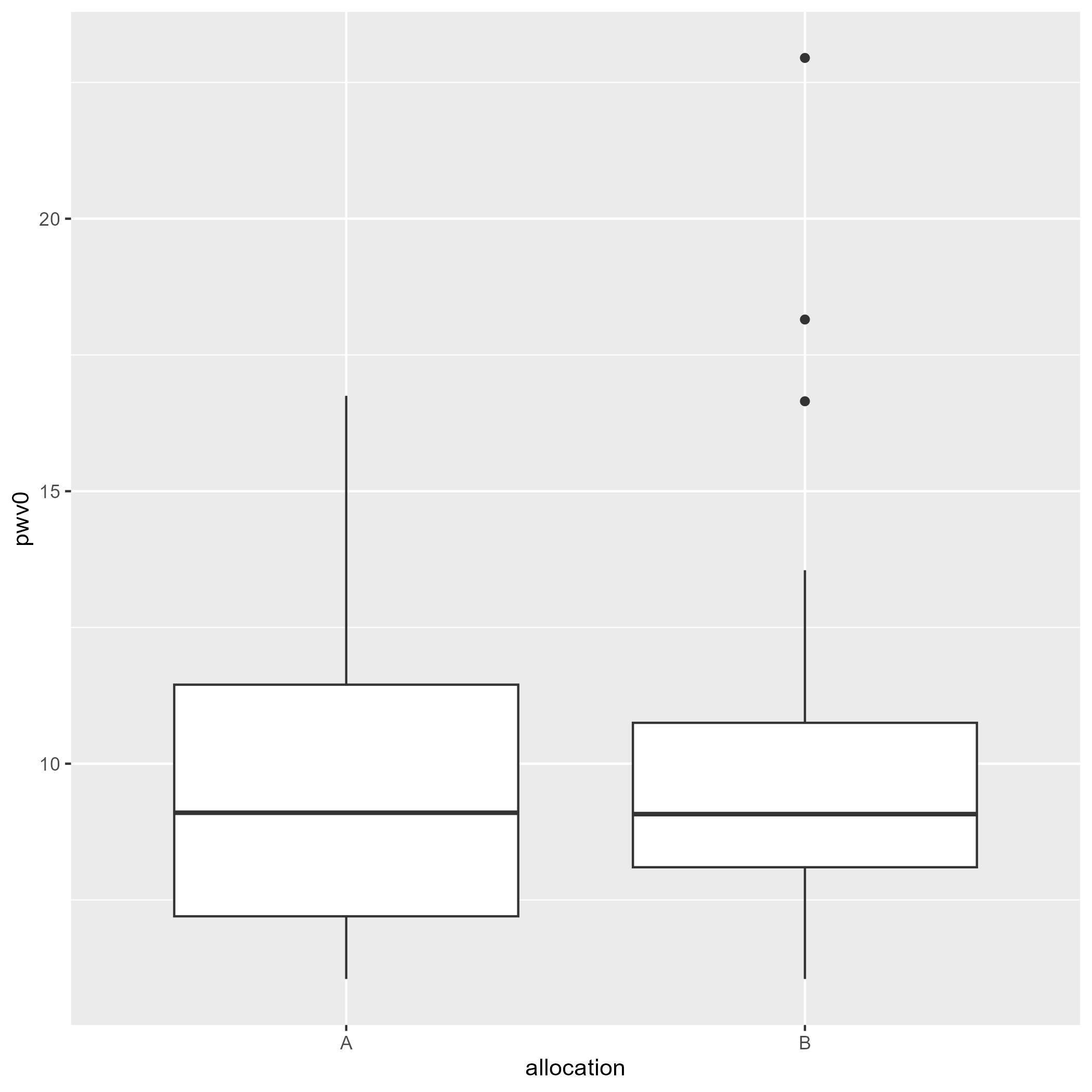
where the following statistical model was used to test the group difference (allocation variable):
> e.lmm <- lmm(pwv0 ~ allocation + sex + age, data = ckdW)
> model.tables(e.lmm)
              estimate         se      df      lower    upper      p.value
(Intercept) -0.6701892 1.98683016 47.0094 -4.6671548 3.326776 7.373804e-01
allocationB  0.3269616 0.82004599 47.0094 -1.3227494 1.976673 6.919113e-01
sexmale      0.8474481 0.95876696 47.0094 -1.0813321 2.776228 3.812519e-01
age          0.1682865 0.03246632 47.0094  0.1029731 0.233600 4.510612e-06
We obtain a mean group difference of 0.327 [-1.323;1.977] instead of 0.266 [-1.806;2.339] had we not have adjusted for sex and age. The previous figure where we display the (raw) outcome per group is therefore not appropriate to illustrate the estimated drug effect. Instead one could provide a graphical representation of the partial residuals:
> plot(e.lmm, type = "partial", variable = "allocation")
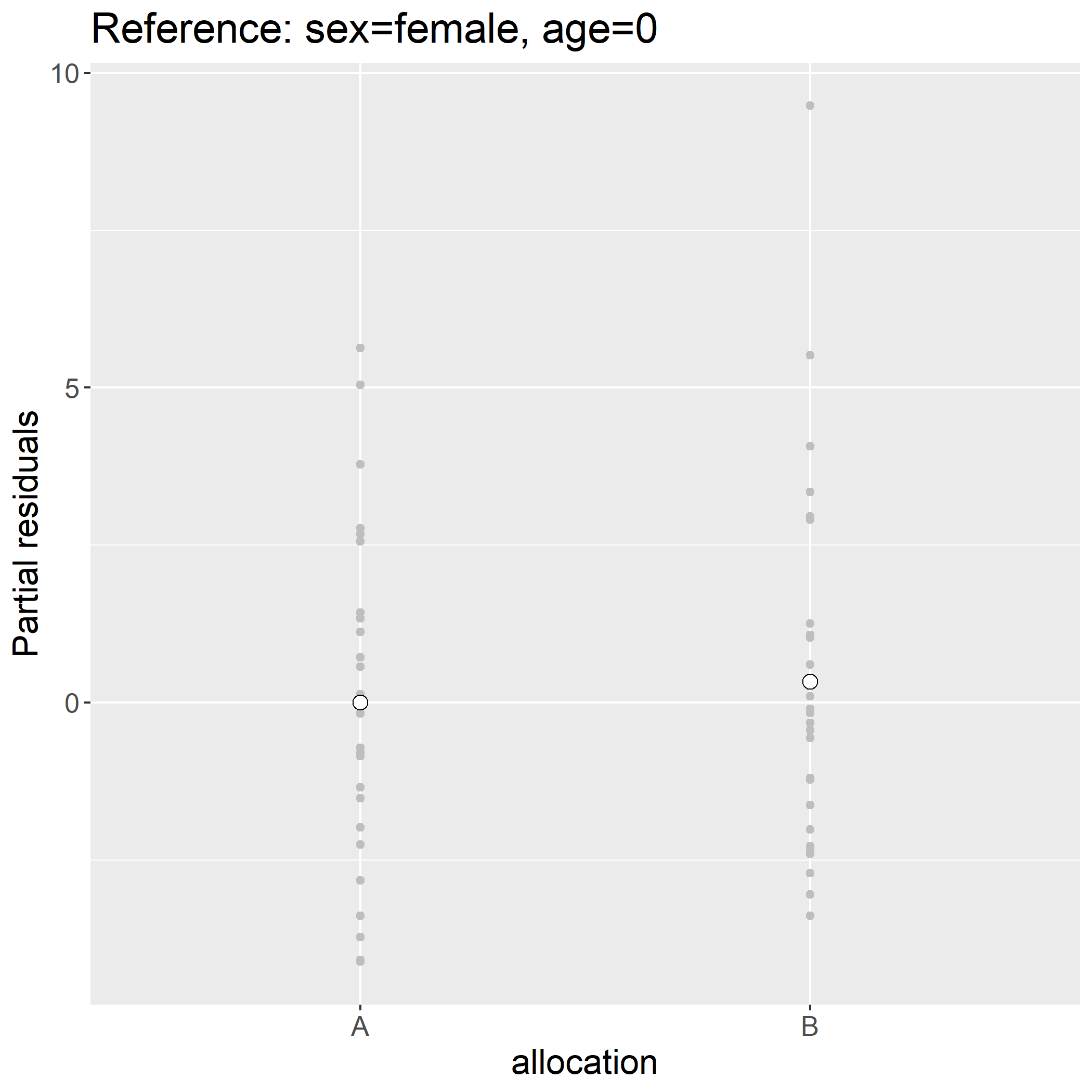
Indead the difference in mean partial residuals between the two groups:
> ckdW$pres <- residuals(e.lmm, type = "partial", variable = "allocation")
> mean(ckdW$pres[ckdW$allocation=="B"]) - mean(ckdW$pres[ckdW$allocation=="A"])
[1] 0.3269616
is exactly the estimated drug effect. One counter-intuitive feature of partial residuals is that there may not follow the original scale (they are typically centered around 0 wherease the outcome value was strictly positive):
> head(ckdW$pres)
[1] -2.7098727 -2.3524574 -1.6281556 -0.1672843 -0.5647286 -2.4024574
Assuming that the model holds, the display is to be understood as the outcome we would have observed had all individuals have had the same sex (here female) and same age (here age 0). Another counter-intuitive feature is that continuous variables have by default reference level 0 which in the case of age is un-realistic. The first issue can be fixed by keeping the intercept (argument var) and the second by specifying the reference levels:
> plot(e.lmm, type = "partial", variable = c("(Intercept)","allocation"),
       at = data.frame(sex = factor("female", levels(ckdW$sex)), age = 58))
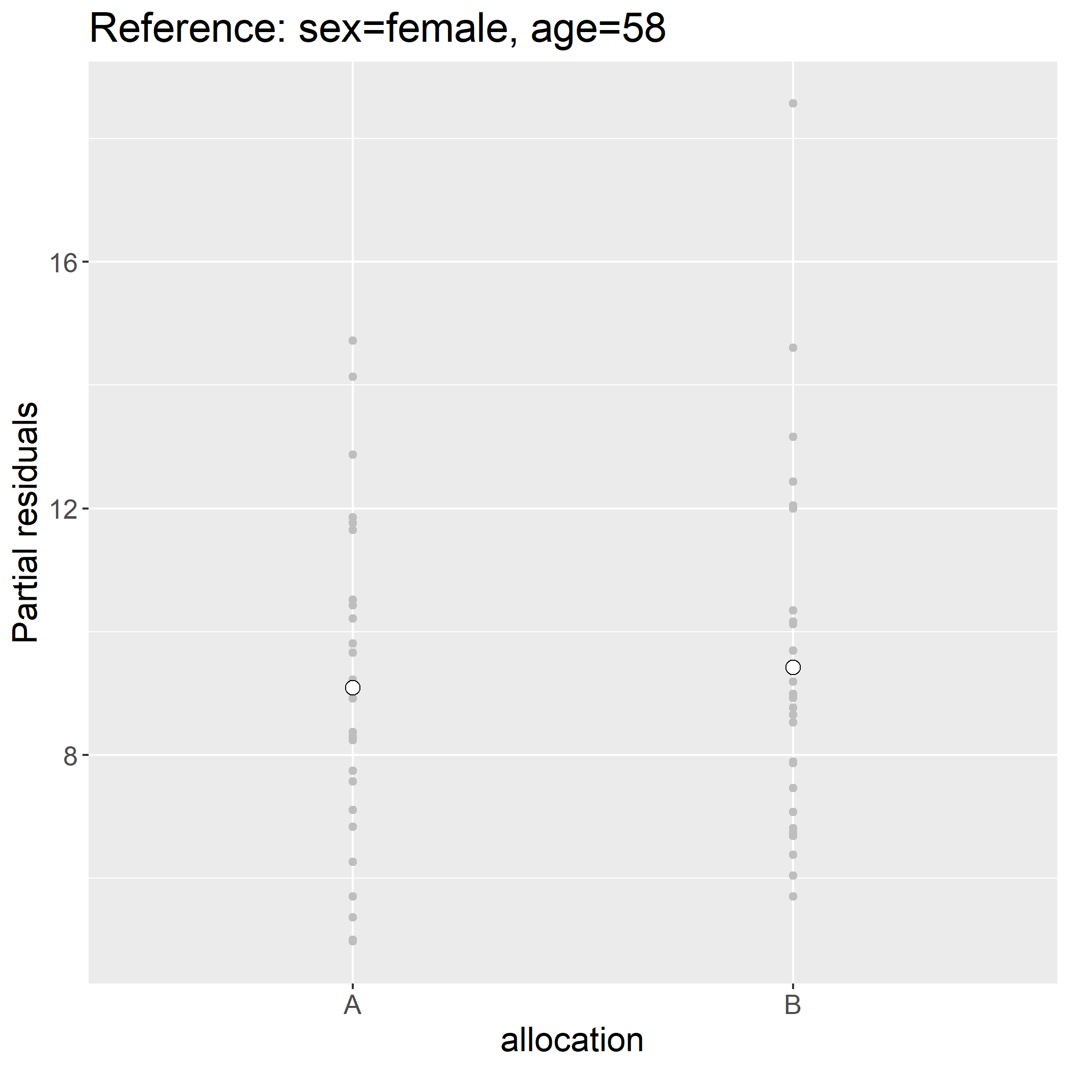
> ckdW$pres.f28 <- residuals(e.lmm, type = "partial", variable = c("(Intercept)","allocation"),
                             at = data.frame(sex = factor("female", levels(ckdW$sex)), age = 58))
> head(ckdW$pres.f28)
[1] 6.380558 6.737973 7.462275 8.923146 8.525702 6.687973
This simplify shift the partial residuals by value, here:
> unique(round(ckdW$pres.f28-ckdW$pres,10))
[1] 9.09043
See the vignette of the LMMstar package for more examples
Greek letters and notations
There is no intrinsic meanning to (\beta), (\rho), … One should define what each refers to in the statistical analysis paragraph. Avoid to use the same letter to refer to two different things. It can be a good idea to use (p) to refer to p-values relative to a single test and (p_{adj}) to FWER adjusted p-values. In the latter case, it should be made clear over which/how many tests the FWER is evaluated.